AI #

A selection of notes that didn’t fit elsewhere or are being worked on!.

Home

Mathematical Foundation

May 28, 2026

AI, ML

Machine Learning, Mathematics, Linear Algebra, Probability, Statistics, Calculus

Mathematical Foundations for Machine Learning #

Machine Learning is built on mathematical principles that allow models to:

represent data
learn patterns
optimise performance

flowchart LR
    DATA[Data]
    MATH[Math Models]
    OPT[Optimisation]
    MODEL[Trained Model]

    DATA --> MATH
    MATH --> OPT
    OPT --> MODEL

ML requires core mathematical tools to understand how ML algorithms work internally. Algebra deals with relationships between variables and quantities, while Calculus focuses on change and optimization.

Formula Sheet

March 12, 2026

AI, Statistics

AI, Statistics, Probability, Revision

Formula Sheet #

This page is a quick reference of definitions + formulas, grouped by the modules.

Notation #

Sample size: \( n \) (sample), \( N \) (population)
Sample mean: \( \bar{x} \) , population mean: \( \mu \)
Sample variance: \( s^2 \) , population variance: \( \sigma^2 \)
Sample SD: \( s \) , population SD: \( \sigma \)
Complement: \( A^c \)
Intersection (“and”): \( A\cap B \) , union (“or”): \( A\cup B \)
Conditional probability: \( P(A\mid B) \)

1. Basic Probability & Statistics #

1.1 Measures of Central Tendency #

Arithmetic mean #

Sample mean (ungrouped):

Supervised Learning

January 3, 2026

AI, ML

Supervised Learning #

Trained using labelled data.
Each example in the training set includes the correct output.
The algorithm learns to generalise and make predictions on unseen data.
Generally more accurate than unsupervised methods.
Requires human intervention for labelling and setup.
Widely used due to its accuracy and efficiency.
Produces highly accurate results when trained on good-quality labelled data.

Classification #

Output is discrete (e.g. Yes/No, Spam/Not Spam).
Used for categorising data into predefined classes.
Support Vector Machine (SVM) is a common classifier (a linear classifier with margin-based separation).

Differentiation of Univariate Functions

AI, ML

Machine Learning, Mathematics, Vector Calculus

Differentiation of Univariate Functions #

Differentiation measures rate of change.

For a function f(x), the derivative measures the rate of change.

\[ f'(x) = \lim_{h \to 0} \frac{f(x+h)-f(x)}{h} \]

Interpretation:

Slope of tangent
Instantaneous rate of change

Home | Vector Calculus

Artificial Intelligence

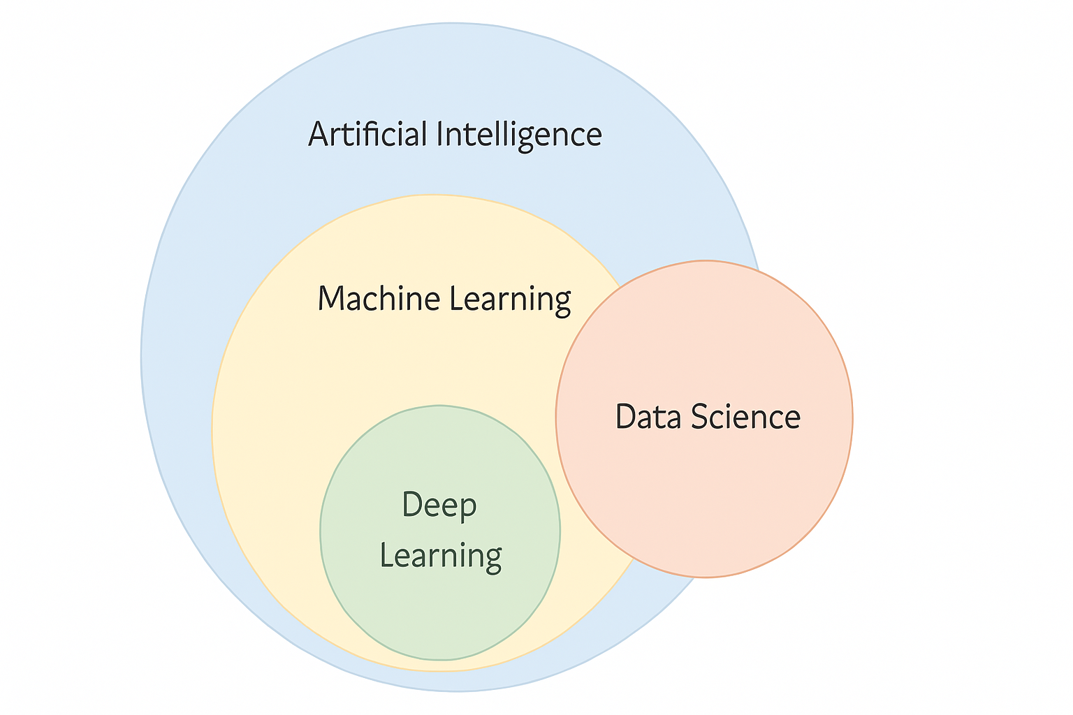
July 4, 2024

AI

My AI Notes #

Learning how machines learn! My working notes as I learn AI.

flowchart LR
    AI[Artificial Intelligence]
    ML[Machine Learning]
    DL[Deep Learning]
    FM[Foundation Models]
    LLM[LLM Models]

    AI --> ML
    ML --> DL
    DL --> FM
    FM --> LLM

    style AI fill:#E1F5FE
    style ML fill:#C8E6C9
    style DL fill:#90CAF9
    style FM fill:#64B5F6
    style LLM fill:#FFCCBC

Mathematical Foundations for Machine Learning
Statistical Methods
Machine Learning
Deep Neural Networks

Machine Learning → The broad field where systems learn patterns from data to make predictions or decisions.
Neural Networks → A subset of machine learning that uses interconnected artificial neurons to model complex relationships.
Deep Learning → A subset of neural networks that uses many hidden layers to learn high-level features from large datasets.
Foundation Models → Large deep learning models trained on massive datasets and reused across many tasks using transfer learning.
LLMs (Large Language Models) → A specialised type of foundation model focused on understanding and generating human language.

flowchart TD
AI["Artificial<br/>Intelligence"]
ML["Machine<br/>Learning"]
NN["Neural<br/>Networks"]
DL["Deep<br/>Learning"]
FM["Foundation<br/>Models"]
LLM["LLM<br/>Models"]

AI --> ML
ML --> NN
NN --> DL
DL --> FM
FM --> LLM

LR["Linear<br/>Regression"]
DT["Decision<br/>Trees"]
ML --> LR
ML --> DT

MLP["MLP"]
CNN["CNN"]
NN --> MLP
NN --> CNN

CNNDL["CNN<br/>(deep)"]
RNN["RNN"]
DL --> CNNDL
DL --> RNN

BERT["BERT"]
CLIP["CLIP"]
FM --> BERT
FM --> CLIP

GPT["GPT"]
LLAMA["LLaMA"]
LLM --> GPT
LLM --> LLAMA

TEXT["Text"]
IMAGE["Images"]
AUDIO["Audio"]
VIDEO["Video"]
LLM --> TEXT
LLM --> IMAGE
LLM --> AUDIO
LLM --> VIDEO

style AI fill:#90CAF9,stroke:#1E88E5,color:#000
style ML fill:#90CAF9,stroke:#1E88E5,color:#000
style NN fill:#90CAF9,stroke:#1E88E5,color:#000

style DL fill:#CE93D8,stroke:#8E24AA,color:#000
style FM fill:#CE93D8,stroke:#8E24AA,color:#000

style LLM fill:#C8E6C9,stroke:#2E7D32,color:#000
style LR fill:#C8E6C9,stroke:#2E7D32,color:#000
style DT fill:#C8E6C9,stroke:#2E7D32,color:#000
style MLP fill:#C8E6C9,stroke:#2E7D32,color:#000
style CNN fill:#C8E6C9,stroke:#2E7D32,color:#000
style CNNDL fill:#C8E6C9,stroke:#2E7D32,color:#000
style RNN fill:#C8E6C9,stroke:#2E7D32,color:#000
style BERT fill:#C8E6C9,stroke:#2E7D32,color:#000
style CLIP fill:#C8E6C9,stroke:#2E7D32,color:#000
style GPT fill:#C8E6C9,stroke:#2E7D32,color:#000
style LLAMA fill:#C8E6C9,stroke:#2E7D32,color:#000
style TEXT fill:#C8E6C9,stroke:#2E7D32,color:#000
style IMAGE fill:#C8E6C9,stroke:#2E7D32,color:#000
style AUDIO fill:#C8E6C9,stroke:#2E7D32,color:#000
style VIDEO fill:#C8E6C9,stroke:#2E7D32,color:#000

AI, ML, DL, and Data Science Diagram

Statistics

March 12, 2026

AI, ML

Statistics, Probability, Data Analysis

Statistics #

Statistical methods help you turn raw data into reliable conclusions, while understanding uncertainty, variability, and confidence.

Statistics provides the language and tools for reasoning about data, uncertainty, and inference.

ML needs understanding data behaviour, drawing conclusions, and validating machine learning models.

Collect Data
Present & Organise Data (in a systematic manner)
Alalyse Data
Infer about the Data
Take Decision from the Data

Statistics Topic	What you learn (plain English)	ML Connection
1. Basic Probability & Statistics	Summarise data; understand spread; basic probability rules	Data understanding (EDA), feature sanity checks, detecting outliers, interpreting “average behaviour”
2. Conditional Probability & Bayes	Update probability using new information; Bayes’ rule	Naïve Bayes, Bayesian thinking, posterior probabilities, probabilistic classification
3. Probability Distributions	Model randomness with distributions; expectation/variance/covariance	Likelihood models, noise assumptions (Gaussian), sampling, probabilistic modelling foundations
4. Hypothesis Testing	Sampling, CLT, confidence intervals, significance tests, ANOVA, MLE	A/B testing, evaluating model improvements, significance vs noise, parameter estimation (MLE)
5. Prediction & Forecasting	Correlation, regression, time series (AR/MA/ARIMA/SARIMA etc.)	Linear regression, forecasting, sequential data modelling, baseline predictive modelling
6. GMM & EM	Mixtures of Gaussians; iterative estimation with EM	Unsupervised learning (soft clustering), density estimation, latent-variable models

flowchart TD
  A["Statistical Methods<br/>AIML ZC418"] --> B["1. Basic Probability and Statistics"]
  A --> C["2. Conditional Probability and Bayes"]
  A --> D["3. Probability Distributions"]
  A --> E["4. Hypothesis Testing"]
  A --> F["5. Prediction and Forecasting"]
  A --> G["6. Gaussian Mixture Model and EM"]

  B --> B1["Central Tendency<br/>Mean - Median - Mode"]
  B --> B2["Variability<br/>Range - Variance - SD - Quartiles"]
  B --> B3["Basic Probability Concepts"]
  B3 --> B31["Axioms of Probability"]
  B3 --> B32["Definition of Probability"]
  B3 --> B33["Mutually Exclusive vs Independent"]

  C --> C1["Conditional Probability"]
  C --> C2["Independence (conditional)"]
  C --> C3["Bayes Theorem"]
  C --> C4["Naive Bayes (intro)"]

  D --> D1["Random Variables<br/>Discrete and Continuous"]
  D --> D2["Expectation - Variance - Covariance"]
  D --> D3["Transformations of RVs"]
  D --> D4["Key Distributions"]
  D4 --> D41["Bernoulli"]
  D4 --> D42["Binomial"]
  D4 --> D43["Poisson"]
  D4 --> D44["Normal (Gaussian)"]
  D4 --> D45["t - Chi-square - F (intro)"]

  E --> E1["Sampling<br/>Random and Stratified"]
  E --> E2["Sampling Distributions<br/>CLT"]
  E --> E3["Estimation<br/>Confidence Intervals"]
  E --> E4["Hypothesis Tests<br/>Means and Proportions"]
  E --> E5["ANOVA<br/>Single and Dual factor"]
  E --> E6["Maximum Likelihood"]

  F --> F1["Correlation"]
  F --> F2["Regression"]
  F --> F3["Time Series Basics<br/>Components"]
  F --> F4["Moving Averages<br/>Simple and Weighted"]
  F --> F5["Time Series Models"]
  F5 --> F51["AR"]
  F5 --> F52["ARMA / ARIMA"]
  F5 --> F53["SARIMA / SARIMAX"]
  F5 --> F54["VAR / VARMAX"]
  F --> F6["Exponential Smoothing"]

  G --> G1["GMM<br/>Mixture of Gaussians"]
  G --> G2["EM Algorithm<br/>E-step - M-step"]

  B -.-> C
  C -.-> D
  D -.-> E
  E -.-> F
  F -.-> G

Data - Types #

flowchart TD
	A[(Data)] --> B["Categorical (Qualitative)"]
    A --> C["Numerical (Quantitative)"]

    B --> B1[Nominal]
    B --> B2[Ordinal]

    C --> C1[Discrete]
    C --> C2[Continuous]

    C2 --> C21[Interval]
    C2 --> C22[Ratio]

    %% Styling
    style A fill:#E1F5FE,stroke:#333
    style B fill:#90CAF9,stroke:#333
    style B1 fill:#90CAF9,stroke:#333
    style B2 fill:#90CAF9,stroke:#333
    style C fill:#FFF9C4,stroke:#333
    style C1 fill:#FFF9C4,stroke:#333
    style C2 fill:#FFF9C4,stroke:#333
    style C21 fill:#FFF9C4,stroke:#333
    style C22 fill:#FFF9C4,stroke:#333

Categorical (Qualitative) #
express a qualitative attribute e.g. hair color, eye color

Stats Formula Sheet

February 25, 2026

AI, Statistics

AI, Statistics, Probability, Revision

Stats Formula Sheet #

Keep this page as a quick reference of definitions + formulas.

Notation #

Sample size: \( n \) (sample), \( N \) (population)
Mean: \( \bar{x} \) (sample), \( \mu \) (population)
Variance: \( s^2 \) (sample), \( \sigma^2 \) (population)
Standard deviation: \( s \) (sample), \( \sigma \) (population)

Module 1: Basic Statistics #

Measures of Central Tendency #

Sample mean (ungrouped):

Partial Differentiation and Gradients

AI, ML

Machine Learning, Mathematics, Vector Calculus

Partial Differentiation and Gradients #

For f(x1, x2, …, xn):

[ \frac{\partial f}{\partial x_i} ]

Gradient vector:

[ \nabla f = \begin{bmatrix} \frac{\partial f}{\partial x_1} \ \vdots \ \frac{\partial f}{\partial x_n} \end{bmatrix} ]

Gradient points in direction of steepest ascent.

flowchart LR
    Input --> Function
    Function --> Gradient
    Gradient --> Optimisation

Home | Vector Calculus

Linear Independence

AI, ML

Machine Learning, Mathematics, Linear Algebra

Linear Independence #

A set of vectors is linearly independent if none of them can be written as a linear combination of the others.

\[ c_1\mathbf{v}_1 + \cdots + c_k\mathbf{v}_k = \mathbf{0} \;\Rightarrow\; c_1=\cdots=c_k=0 \]

Independence means each vector adds new information.

AI #

Mathematical Foundations for Machine Learning #

Formula Sheet #

Notation #

1. Basic Probability & Statistics #

1.1 Measures of Central Tendency #

Arithmetic mean #

Supervised Learning #

Classification #

Differentiation of Univariate Functions #

My AI Notes #

Statistics #

Data - Types #

Categorical (Qualitative) #

Stats Formula Sheet #

Notation #

Module 1: Basic Statistics #

Measures of Central Tendency #

Partial Differentiation and Gradients #

Linear Independence #