Higher-order derivatives

Higher-order derivatives #

Home | Vector Calculus

Angles and Orthogonality

Angles and Orthogonality #

Once we define an inner product, we can define the angle between two vectors.

Angles allow us to measure how aligned or different two vectors are in space.

Key Idea: Angle measures similarity between vectors. Orthogonality means complete independence (no similarity).

Why It Matters in Machine Learning #

• PCA produces orthogonal components
• Orthogonal features reduce redundancy
• Gradient directions depend on angle

Angle Formula #

For vectors in n-dimensional space:

Artificial and Computational Intelligence

Artificial and Computational Intelligence #

Artificial and Computational Intelligence studies how agents perceive, reason, search, optimise, learn and act in complex environments.

Core Learning Pages #

Modular Structure #

1. Introduction #

• Artificial Intelligence foundations
• Overview of modern AI
• AI application domains

2. Introduction to Intelligent Agents #

• Notion of agents and environments
• Rationality
• Nature of environments
• Structure of agents

3. Problem-Solving Agents Using Search #

• Problem formulation
• Uninformed and informed search algorithms
• Heuristics
• Greedy Best-First Search
• A* Search and optimality of A*
• Heuristic accuracy and algorithm performance
• Admissible heuristics from relaxed problems
• Pattern databases and experience
• Learning heuristics
• Local search and optimisation
• Hill Climbing
• Local Beam Search
• Genetic Algorithms
• Ant Colony Optimisation
• Neural Architecture Search
• Neuroevolution

4. Game Playing #

• Minimax Algorithm
• Alpha-Beta Pruning
• Monte Carlo Tree Search
• Stochastic Games

5. Knowledge Representation Using Logic #

• Propositional and Predicate Logic
• TT-Entail and theorem proving
• Logic representation of intelligent agents
• Proof by resolution
• DPLL Algorithm
• Agents based on Propositional Logic
• Unification
• Forward Chaining
• Backward Chaining
• Resolution

6. Multi-Agent Decision Making #

• Properties of multi-agent environments
• Multi-agent planning
• Non-Cooperative Game Theory
• Cooperative Game Theory
• Collective decision making

7. Probabilistic Representation and Reasoning #

• Representing knowledge in uncertain domains
• Semantics of Bayesian Networks
• Exact inference in Bayesian Networks
• Approximate inference in Bayesian Networks

8. Probabilistic Reasoning Over Time #

• Time and uncertainty
• Inference in temporal models
• Hidden Markov Models
• Learning HMMs
• Dynamic Bayesian Networks

9. Ethics in AI #

• Explainable AI
• Logically Explained Networks
• Explainable Bayesian Networks

Experiments #

Practical Tools #

• Programming languages: Python, Prolog
• Tools and libraries: Jupyter, NumPy, SciPy, Pandas, pgmpy, NLTK
• Environments: Google Colab, SWI-Prolog Online

Book References #

Primary Textbook #

1. Stuart Russell and Peter Norvig, Artificial Intelligence: A Modern Approach, 4th Edition, Pearson Education, 2020.

Reference Books #

1. Ryszard S. Michalski, Jaime G. Carbonell and Tom M. Mitchell, Machine Learning: An Artificial Intelligence Approach, Elsevier, 2014.
2. Dan W. Patterson, Introduction to AI and Expert Systems, Prentice Hall of India, New Delhi, 2010.
3. Elaine Rich and Kevin Knight, Artificial Intelligence, 2nd Edition, Tata McGraw Hill Publishing Company, New Delhi, 2003.

Home | Artificial Intelligence

Taylor’s series

Linearization and multivariate Taylor’s series #

Home | Vector Calculus

Maxima and Minima

Computing maxima and minima for unconstrained optimization #

Home | Vector Calculus

AI Stages: ANI, AGI, ASI

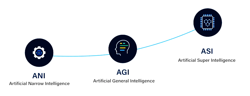
July 4, 2024

AI Development Stages: ANI → AGI → ASI #

Artificial Intelligence is often described in three stages, based on capability and scope:

• ANI: Task-specific intelligence (today’s AI)
• AGI: Human-level general intelligence (future goal)
• ASI: Beyond human intelligence (theoretical)

ANI — Artificial Narrow Intelligence #

• also called Weak AI
• designed to perform one specific task
• Operates within a predefined environment
• Cannot generalise beyond its training
• Most AI systems today are ANI

examples

Artificial Intelligence

Artificial Intelligence #

Artificial Intelligence (AI) is concerned with building systems that can perceive, reason, learn, decide and act in ways that achieve useful goals.

This page introduces the foundations of AI, its major application areas, four classic ways of thinking about intelligence, important milestones in its development, and some of the risks that accompany increasingly capable AI systems.

• Artificial Intelligence: Foundations, Overview of Modern AI & Application Domains.
• What is Artificial Intelligence: Acting Humanly, Thinking humanly, Thinking rationally, Acting Rationally
• Foundations of AI , Brief Overview of Modern AI & Application Domains

Learning Objectives #

• explain what intelligence and artificial intelligence mean in practical terms
• identify the major disciplines that contributed to AI
• distinguish thinking humanly, acting humanly, thinking rationally and acting rationally
• explain the idea behind the Turing Test
• describe why the rational-agent view is central to modern AI
• recognise important application areas and risks of AI

Big Picture #

flowchart TD
    A["Artificial Intelligence"] --> B["Human-like"]
    A --> C["Rational"]
    B --> D["Think like humans"]
    B --> E["Act like humans"]
    C --> F["Think rationally"]
    C --> G["Act rationally"]

    style A fill:#C8E6C9
    style B fill:#E1F5FE
    style C fill:#FFF9C4
    style D fill:#EDE7F6
    style E fill:#EDE7F6
    style F fill:#C8E6C9
    style G fill:#C8E6C9

1. What Is Intelligence? #

Intelligence is not a single ability. It involves several capabilities working together, including:

Basic Statistics

Basic Statistics #

Statistics: describes data (what you see).
Probability: models uncertainty (what you don’t know yet).

• Summarise a dataset using central tendency and variability
• Explain core probability ideas using simple examples
• Apply the axioms of probability
• Distinguish mutually exclusive vs independent events

flowchart TD
    A[Dataset] --> B[Central Tendency]
    A --> C[Variability]
    B --> B1[Mean]
    B --> B2[Median]
    B --> B3[Mode]
    C --> C1[Range]
    C --> C2[Variance]
    C --> C3[Standard Deviation]
    C --> C4[IQR]

Measures of Central Tendency #

Central tendency tells you where the “middle” of the data is. Describes a set of scores with a single number that describes the PERFORMANCE of the group.

M1: Foundations

M1: Foundations #

This module establishes how to measure ML system performance, identify bottlenecks, and decide which work can run in parallel. It connects algorithmic complexity with the capabilities and limits of CPUs, GPUs, and clusters.

Module coverage:

• Performance Metrics and Complexity Analysis: time and space complexity, throughput, latency, and speedup through Amdahl’s Law.
• Parallelisation Paradigms: data-level, task-level, and algorithm-specific parallelism.
• Modern Hardware Architectures: multi-core CPUs, GPGPUs, GPU/CPU clusters, and resource management.

Learning Objectives #

• Distinguish complexity from measured running time, throughput, and latency.
• Explain the limits of speedup and the cost of communication.
• Choose between data, task, and request parallelism for a workload.
• Relate memory hierarchy, bandwidth, and hardware organisation to performance.

Pages #

Topic Outline #

1. ML and DL System Performance #

• Time complexity of algorithms and running time
• Performance scaling and tuning
• Training versus deployment
• Distributed and cloud environments, embedded devices, and mobile systems
• Throughput and response time

2. Parallel and Distributed Algorithms #

• Systems and performance
• Speedup: approaches, issues, and Amdahl’s Law ☆
• Data parallelism, task parallelism, and request parallelism
• Scale-out clusters: communication cost and its impact on speedup
• Scale-up versus scale-out

3. Parallel Programming Models #

• Parallel programming models and the MapReduce pattern
• Task-parallel and request-parallel execution
• Multi-core and GPGPU parallelism: SIMD versus MIMD
• Memory hierarchies and bandwidth considerations
• CPU-only and GPU-accelerated distributed clusters
• Horizontal and vertical data sharding
• Parameter-server and all-reduce paradigms

How This Module Connects #

Performance measurement and parallel execution provide the basis for M2: Distributed ML Algorithms. Communication and memory limits remain relevant throughout the later modules.

ML and DL System Performance

ML and DL System Performance #

Machine learning system optimisation begins with measurement. Before changing an algorithm, adding processors, or moving work to a GPU, we need to understand what is slow, which resource is limiting performance, and how performance changes as the workload grows.

Course coverage:

1. Metrics: time complexity, running time, space, throughput, latency, and response time
2. Performance scaling and tuning: measuring bottlenecks and predicting how a workload grows
3. Training versus deployment: different objectives, workloads, and constraints
4. Deployment environments: distributed and cloud systems, embedded devices, and mobile systems

Learning Objectives #

By the end of this page, you should be able to: