AI

Gradient Descent and Mini-Batch Gradient Descent

Optimisation: Gradient Descent and Mini-Batch Gradient Descent #

Gradient descent is the core optimisation idea behind neural network training. It updates the model parameters by moving in the opposite direction of the gradient of the loss.

Key takeaway:
Gradient descent uses the gradient to decide how to change the parameters. The learning rate controls how large each update step is.


flowchart TD
    A["Gradient Descent Variants"] --> B["Batch Gradient Descent"]
    A --> C["Stochastic Gradient Descent"]
    A --> D["Mini-batch Gradient Descent"]

    B --> B1["Uses full dataset"]
    B --> B2["One update per epoch"]
    B --> B3["Smooth but slow"]

    C --> C1["Uses one example at a time"]
    C --> C2["Frequent updates"]
    C --> C3["Fast but noisy"]

    D --> D1["Uses small batches"]
    D --> D2["Efficient on hardware"]
    D --> D3["Balanced and practical"]

    style A fill:#E1F5FE,stroke:#4A90E2,stroke-width:2px
    style B fill:#EDE7F6,stroke:#7E57C2
    style C fill:#C8E6C9,stroke:#43A047
    style D fill:#FFF9C4,stroke:#FBC02D

Gradient Descent Rule ☆ #

The gradient tells us the direction in which the loss increases fastest. To reduce the loss, we move in the opposite direction.

Momentum Methods

Optimisation: Momentum Methods #

Momentum improves gradient descent by adding a memory of previous update directions. Instead of using only the current gradient, the optimiser accumulates velocity across iterations.

Key takeaway:
Momentum helps the optimiser move faster in consistent directions and reduces zigzag movement in directions where gradients oscillate.


flowchart TD
    A["Momentum-based Optimiser"] --> B["SGD with Momentum"]

    B --> B1["Adds velocity term"]
    B --> B2["Accumulates past gradients"]
    B --> B3["Reduces zig-zag movement"]
    B --> B4["Speeds up movement in useful direction"]
    B --> B5["Helps through shallow regions"]

    B1 --> C1["Current update depends on previous update"]
    B2 --> C2["Builds inertia"]
    B3 --> C3["Smoother path to minimum"]

    style A fill:#C8E6C9,stroke:#43A047,stroke-width:2px
    style B fill:#E1F5FE,stroke:#4A90E2
    style B1 fill:#EDE7F6,stroke:#7E57C2
    style B2 fill:#FFF9C4,stroke:#FBC02D
    style B3 fill:#F8BBD0,stroke:#D81B60
    style B4 fill:#EDE7F6,stroke:#7E57C2
    style B5 fill:#FFF9C4,stroke:#FBC02D

Physical Intuition ☆ #

Momentum is often explained using the analogy of a ball rolling down a hill.

Regularisation for Deep models

Regularisation for Deep models #

Regularisation means adding constraints or techniques that prevent a model from becoming too complex and memorising the training data.

The goal is not only low training error.

The goal is good performance on unseen data.

Key takeaway:
Regularisation helps the model generalise by controlling complexity, stabilising training, and reducing overfitting.

  • Generalization for regression
  • Training Error and Generalization Error
  • Underfitting or Overfitting
  • Model Selection
  • Weight Decay and Norms
  • Generalization in Classification
  • Environment and Distribution Shift
  • Generalization in Deep Learning
  • Dropout
  • Batch Normalization
  • Layer Normalization

Underfitting, Good Fit, and Overfitting ☆ #

CaseModel behaviourTraining errorTest error
Underfittingtoo simplehighhigh
Good fitcaptures useful patternlowlow
Overfittingmemorises training noisevery lowhigh
flowchart LR
    A["Model Complexity"] --> B["Too Simple: Underfitting"]
    A --> C["Just Right: Good Fit"]
    A --> D["Too Complex: Overfitting"]

    style A fill:#E1F5FE,stroke:#4A90E2
    style B fill:#FFF9C4,stroke:#FBC02D
    style C fill:#C8E6C9,stroke:#43A047
    style D fill:#EDE7F6,stroke:#7E57C2

Training Error and Generalisation Error ☆ #

Training error measures performance on data used for learning.

Linear Algebra

Linear Algebra #

The study of vectors and matrices is called Linear Algebra.

Linear Algebra provides the mathematical language used to represent data, transformations, and structure in ML.


Why Linear Algebra Matters in ML #

  • Every machine learning model uses matrices
  • All data in ML is represented using vectors and matrices
  • Neural networks are pipelines of matrix operations
  • Models apply matrix transformations to data
  • Optimisation relies on linear algebra operations

What to Learn #

  • Scalars, vectors, and matrices
  • Vector operations (addition, dot product)
  • Matrix multiplication (critical)
  • Identity matrices and transpose
  • Eigenvalues and eigenvectors (conceptual understanding)

  • Scalar → a number
  • Vector → a directed point
  • Matrix → a space transformer
  • Linear transformation → structured mapping
  • Feature → one axis
  • Feature space → where data lives
  • Vector space → where vectors live

Home | Mathematical Foundation

Linear Systems

Linear Systems #

How systems of linear equations are represented and solved using matrices.

  • the study of vectors and rules to manipulate vectors
  • describe multiple linear equations solved simultaneously
  • connect algebraic equations with matrix representations

Matrix


Idea of Closure #

  • performing a specific operation (like addition or multiplication) on members of a set always produces a result that belongs to the same set

  • idea of closure is fundamental to defining a Vector space because it ensures that performing arithmetic operations (addition and scalar multiplication) on vectors within a set does not produce a new element outside that set.

Systems of Linear Equations

Systems of Linear Equations #

A system of linear equations can be written compactly as:

\[ A\mathbf{x}=\mathbf{b} \]

This represents:

  • a linear transformation applied to an unknown vector (\mathbf{x})
  • producing an output vector (\mathbf{b})

Key components #

Coefficient matrix (A) #

(A) contains the coefficients of the variables.

Calculus

Calculus #

Calculus is:

  • the mathematical framework for understanding and controlling how quantities change
  • the mathematics of change and accumulation

It helps answer:

  • How fast is something changing right now?
  • What happens when inputs change slightly?
  • Where is something maximum or minimum?

It answers two big questions:

  • How fast is something changing right now? → derivatives (differentiation)
  • How much has accumulated over an interval? → integrals (integration)

flowchart TD
  A[Calculus] --> B[Limits]
  B --> C[Continuity]
  B --> D[Derivatives]
  B --> E[Integrals]
  D --> F[Optimisation: maxima/minima]
  D --> G[ML: gradients & learning]
  E --> H[Accumulation: area/total change]


  1. Differential Calculus (Rates of Change) #

    Studies how things change.

Matrices

Matrices #

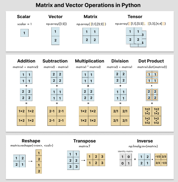
Matrices are the core data structure of linear algebra and the workhorse of machine learning.
Almost every ML model can be described as a sequence of matrix operations.


Matrix #

A matrix is a rectangular array of numbers arranged in rows and columns.

\[ A \in \mathbb{R}^{m \times n} \]

An ( m \times n ) matrix has:

Solving Linear Systems

Solving Linear Systems #

Solve using:

  • Substitution Method
  • Elimination Method (Multiple & then Subtract)
  • Cross Multiplication

Linear system can have:

  • no solution
  • a unique solution
  • infinitely many solutions

Positive Definite Matrices #

A square matrix is positive definite if pre-multiplying and post-multiplying it by the same vector always gives a positive number as a result, independently of how we choose the vector.

Positive definite symmetric matrices have the property that all their eigenvalues are positive.