 July 4, 2024
AI Development Stages: ANI → AGI → ASI
#
Artificial Intelligence is often described in three stages, based on capability and scope:
- ANI: Task-specific intelligence (today’s AI)
- AGI: Human-level general intelligence (future goal)
- ASI: Beyond human intelligence (theoretical)
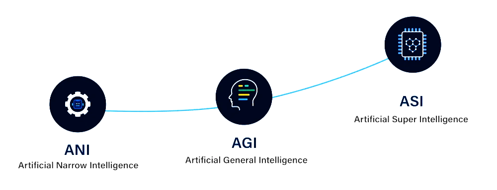
ANI — Artificial Narrow Intelligence
#
- also called Weak AI
- designed to perform one specific task
- Operates within a predefined environment
- Cannot generalise beyond its training
- Most AI systems today are ANI
examples
M1: Foundations
#
This module establishes how to measure ML system performance, identify bottlenecks, and decide which work can run in parallel. It connects algorithmic complexity with the capabilities and limits of CPUs, GPUs, and clusters.
Module coverage:
- Performance Metrics and Complexity Analysis: time and space complexity, throughput, latency, and speedup through Amdahl’s Law.
- Parallelisation Paradigms: data-level, task-level, and algorithm-specific parallelism.
- Modern Hardware Architectures: multi-core CPUs, GPGPUs, GPU/CPU clusters, and resource management.
Learning Objectives
#
- Distinguish complexity from measured running time, throughput, and latency.
- Explain the limits of speedup and the cost of communication.
- Choose between data, task, and request parallelism for a workload.
- Relate memory hierarchy, bandwidth, and hardware organisation to performance.
Pages
#
| Chapter | Page | Main focus |
|---|
| 1 | ML and DL System Performance | Complexity, performance metrics, scaling, tuning, training and deployment |
| 2 | Parallel and Distributed Algorithms | Speedup, Amdahl’s Law, parallelism types, scale-up and scale-out |
| 3 | Parallel Programming Models | MapReduce, multi-core CPUs, GPGPUs, memory hierarchy, and clusters |
Topic Outline
#
- Time complexity of algorithms and running time
- Performance scaling and tuning
- Training versus deployment
- Distributed and cloud environments, embedded devices, and mobile systems
- Throughput and response time
2. Parallel and Distributed Algorithms
#
- Systems and performance
- Speedup: approaches, issues, and Amdahl’s Law ☆
- Data parallelism, task parallelism, and request parallelism
- Scale-out clusters: communication cost and its impact on speedup
- Scale-up versus scale-out
3. Parallel Programming Models
#
- Parallel programming models and the MapReduce pattern
- Task-parallel and request-parallel execution
- Multi-core and GPGPU parallelism: SIMD versus MIMD
- Memory hierarchies and bandwidth considerations
- CPU-only and GPU-accelerated distributed clusters
- Horizontal and vertical data sharding
- Parameter-server and all-reduce paradigms
How This Module Connects
#
Performance measurement and parallel execution provide the basis for M2: Distributed ML Algorithms. Communication and memory limits remain relevant throughout the later modules.
Machine learning system optimisation begins with measurement. Before changing an algorithm, adding processors, or moving work to a GPU, we need to understand what is slow, which resource is limiting performance, and how performance changes as the workload grows.
Course coverage:
- Metrics: time complexity, running time, space, throughput, latency, and response time
- Performance scaling and tuning: measuring bottlenecks and predicting how a workload grows
- Training versus deployment: different objectives, workloads, and constraints
- Deployment environments: distributed and cloud systems, embedded devices, and mobile systems
Learning Objectives
#
By the end of this page, you should be able to:
Reinforcement Learning
#
Reinforcement Learning (RL) is a learning approach in which an agent improves its behaviour by interacting with an environment and observing the rewards produced by its actions.
Unlike supervised learning, the agent is not given a correct action label for every situation. It must discover useful behaviour through trial, feedback, and repeated interaction.
Reinforcement learning is goal-oriented learning through interaction.
Why Reinforcement Learning?
#
RL is useful when decisions affect what happens next and the quality of an action may only become clear later.
Neural Networks
#
- A network of artificial neurons inspired by how neurons function in the human brain.
- At its core - a mathematical model designed to process and learn from data.
- Neural networks form the foundation of Deep Learning (involves training large and complex networks on vast amounts of data).
flowchart LR
 subgraph subGraph0["Input Layer"]
        I1(("Input 1"))
        I2(("Input 2"))
        I3(("Input 3"))
  end
 subgraph subGraph1["Hidden Layer"]
        H1(("Hidden 1"))
        H2(("Hidden 2"))
        H3(("Hidden 3"))
  end
 subgraph subGraph2["Output Layer"]
        O(("Output"))
  end
    I1 --> H1 & H2 & H3
    I2 --> H1 & H2 & H3
    I3 --> H1 & H2 & H3
    H1 --> O
    H2 --> O
    H3 --> O

    style I1 fill:#C8E6C9
    style I2 fill:#C8E6C9
    style I3 fill:#C8E6C9
    style H1 stroke:#2962FF,fill:#BBDEFB
    style H2 fill:#BBDEFB
    style H3 fill:#BBDEFB
    style O fill:#FFCDD2
    style subGraph0 stroke:none,fill:transparent
    style subGraph1 stroke:none,fill:transparent
    style subGraph2 stroke:none,fill:transparent
Structure of a Neural Network
#
A typical neural network has three main layers:
Artificial Neuron and Perceptron
#
knowledge in neural networks is stored in connection weights, and learning means modifying those weights.
Biological Neuron
#
A biological neuron is a specialised cell that processes and transmits information through electrical and chemical signals.
Core components:
- Dendrites: receive signals from other neurons
- Cell body (soma): processes incoming signals
- Axon: transmits the output signal
- Synapses: connection points between neurons
Biological intuition:
- many inputs arrive to one neuron
- one neuron can connect out to many neurons
- massive parallelism enables fast perception and recognition
Artificial Neuron
#
An artificial neuron is a simplified computational model inspired by biological neurons.
M2: Distributed ML Algorithms
#
This module applies parallel and distributed computing to ML algorithms. It examines how to divide computation, combine results, and balance communication against useful work during training.
Module coverage:
- Parallel ML Algorithms: CNNs, gradient descent and SGD, SVM, k-means, k-nearest neighbours, decision trees, and random forests.
- Distributed Training Strategies: data parallelism, model parallelism, pipeline parallelism, gradient checkpointing, and mixed-precision training.
Learning Objectives
#
- Decompose ML algorithms into independent and dependent work.
- Explain how local results are aggregated and where communication is required.
- Compare distributed execution through Hadoop and Spark.
- Choose training strategies that address compute and memory constraints.
Pages
#
| Chapter | Page | Main focus |
|---|
| 4 | Parallelisation of ML Algorithms | Problem decomposition, ensembles, XGBoost, k-means, trees, forests, and SVM |
| 5 | Communication-Aware Distributed ML | Communication overhead, distributed k-means and k-NN, model parallelism, and SGD |
| 6 | Clusters, Hadoop, and Spark | Cluster frameworks, MapReduce k-means, distributed CNNs, and communication reduction |
| 7 | Distributed Training Strategies | Data, model, and pipeline parallelism, checkpointing, and mixed precision |
Topic Outline
#
4. Parallelisation of ML Algorithms
#
- Problem decomposition and parallelisation
- Ensemble methods and XGBoost on CPUs
- k-means
- Distributed decision trees and random forests
- Distributed implementations using Spark ML and XGBoost
- Parallel SVM kernel computation using block-wise and MapReduce-style methods
5. Communication-Aware Distributed ML
#
- Communication overhead in distributed algorithms
- Distributed k-means and model parallelism
- k-NN: data partitioning, locality-sensitive hashing, and distributed indexing
- KD-tree and Ball-tree indexing versus brute-force MapReduce
- Accuracy–latency trade-offs in approximate k-NN
- Gradient descent and SGD: mini-batch, synchronous, and asynchronous variants
6. Clusters, Hadoop, and Spark
#
- Cluster computing with Hadoop and Spark
- Lloyd’s k-means algorithm in MapReduce
- Mini-batch k-means and streaming variants
- Convergence criteria and communication reduction through compressed updates
- CNN data and model parallelism, including layer splitting and tensor slicing
- Mixed precision, pipeline parallelism, and distributed training frameworks
7. Distributed Training Strategies ☆
#
- Data parallelism
- Model parallelism
- Pipeline parallelism
- Gradient checkpointing
- Mixed-precision training
How This Module Connects
#
Use M1: Foundations to interpret complexity and speedup. Continue to M3: Scale-Out Systems for the platforms and communication mechanisms that support larger training runs.
Machine learning Workflow
#
Data is the foundation of any machine learning system.
Quality of data matters more than model complexity.
Role of Data
#
Data determines:
- What patterns the model can learn
- How well it generalises
- Whether bias or noise is introduced
Bad data → bad model (even with perfect algorithms).
Data Preprocessing, wrangling
#
Raw data is never ready for training.
Data Issues
- Noise
- For objects, noise is an extraneous object
- For attributes, noise refers to modification of original values
- Use Log or Z Transfer to convert to mean
- Outliers
- Data objects with characteristics that are considerably different than most of the other data objects in the data set
- Handle: Use IQR method
- Find Lower and Upper Bound and replace Outlier with Lower or Upper Bound
- Missing Values
- Eliminate data objects or variables
- Handle: Estimate missing values
- Mean, Median or Mode
- Prefer Median if there are missing outliers
- Ignore the missing value during analysis
- Duplicate Data
- Major issue when merging data from heterogeneous sources
- Inconsistent Codes
- Find all Unique and transfer all inconsistent to
Data Preprocessing techniques
Multi-Armed Bandit Problem
#
The Multi-Armed Bandit (MAB) problem is the simplest setting for studying decision-making under uncertainty.
An agent repeatedly chooses one of
\( k \)
actions. Each action produces a numerical reward drawn from an unknown distribution. The objective is to maximise the expected total reward over time.
The central challenge is deciding when to exploit current knowledge and when to explore uncertain alternatives.- Multi-armed Bandit Problem - Motivation and Problem Statement
- Incremental solution to the stationary & non-stationary MAB problems
- Exploration vs. Exploitation trade-off
- Bandit Gradient Algorithm as Stochastic Gradient Ascent
- Associative Search
The k-Armed Bandit Problem ☆
#
At every time step:
Parallel and Distributed Algorithms
#
Parallelisation divides computational work into parts that can execute concurrently. The purpose is to reduce completion time or increase throughput, but the gain depends on how much work is genuinely independent and how much overhead is introduced.
Course coverage:
- Systems and performance: execution time, throughput, efficiency, and bottlenecks
- Speedup—approaches and issues: Amdahl’s Law, serial work, overhead, and load imbalance
- Data parallelism versus task parallelism versus request parallelism
- Scale-out clusters: communication cost and its impact on speedup
The worked algorithms also show how divide-and-conquer and matrix operations expose parallel work.