Cost Function #

also known as an objective function
measure of the difference between predicted values and actual values
quantifies the error between a model’s predicted values and actual values
measures the model’s error on a group of datapoints
method used to predict values by drawing the best-fit line through the data
used to evaluate the accuracy of a model’s predictions
guides the process of adjusting the model’s parameters in order to minimise the difference between predicted and actual values

flowchart TD
CF["Cost<br/>function"] -->|measures| ERR["Prediction<br/>error"]
CF -->|guides| OPT["Optimisation<br/>(training)"]

CF -->|includes| DATA["Data<br/>fit"]
CF -->|may include| PEN["Penalty<br/>(regularisation)"]

style CF fill:#90CAF9,stroke:#1E88E5,color:#000

style ERR fill:#CE93D8,stroke:#8E24AA,color:#000
style OPT fill:#CE93D8,stroke:#8E24AA,color:#000

style DATA fill:#C8E6C9,stroke:#2E7D32,color:#000
style PEN fill:#C8E6C9,stroke:#2E7D32,color:#000

Key takeaway: In ML, we choose model parameters to minimise a cost $J$. For linear regression, the most common choice is the squared error cost.

Training set and model #

You have a training set with:

input features $x$
output targets $y$

The linear regression model is:

\[ f_{w,b}(x)=wx+b \]

The values $w$ and $b$ are the parameters of the model. You adjust them during training to improve the model.

You may also hear:

$w,b$ called coefficients
$w,b$ called weights

What w and b do #

Different values of $w$ and $b$ give different straight lines.

$b$ is the y-intercept: the value of the prediction when $x=0$
$w$ is the slope: how much the prediction changes when $x$ increases

Examples:

If $w=0$ and $b=1.5$: the model predicts a constant $1.5$ (horizontal line)
If $w=0.5$ and $b=0$: the line passes through the origin and has slope $0.5$
If $w=0.5$ and $b=1$: same slope, shifted up by 1

Predictions on training examples #

A training example is written as: $(x^{(i)},y^{(i)})$

For input $x^{(i)}$, the model predicts:

\[ \hat{y}^{(i)} = f_{w,b}\!\left(x^{(i)}\right)=wx^{(i)}+b \] $f_{w,b}\!\left(x^{(i)}\right)$ : our prediction for example $i$ using parameters $w,b$

Goal: choose $w$ and $b$ so that $\hat{y}^{(i)}$ is close to $y^{(i)}$ for many (ideally all) training examples.

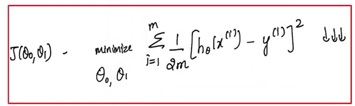
Computing Cost #

Equation for cost with one variable is:

\[ J(w,b)=\frac{1}{2m}\sum_{i=0}^{m-1}\left(f_{w,b}\!\left(x^{(i)}\right)-y^{(i)}\right)^2 \] $\left(f_{w,b}\!\left(x^{(i)}\right)-y^{(i)}\right)^2$ : the squared difference between the target value and the prediction

The squared differences are summed over all the $m$ examples and divided by $2m$ to produce the cost $J(w,b)$

Cost Fn

Intuition: error and squared error #

For one example $i$, the error is:

\[ \hat{y}^{(i)}-y^{(i)} \]

Squared error for example $i$:

\[ \left(\hat{y}^{(i)}-y^{(i)}\right)^2 \]

The cost function sums squared errors over the dataset and averages them (via $2m$).

Squared Error & Mean Squared Error (MSE) #

Feature	Squared Error	Mean Squared Error (MSE)
Scope	Individual data point (residual)	Entire dataset
Formula	$ (y_i - \hat{y}_i)^2 $	$ \frac{1}{n}\sum_{i=1}^{n}(y_i - \hat{y}_i)^2 $
Output	One value per observation	One single value for the model
Purpose	Measures individual error	Measures overall model performance

Cost surface visualisation #

Simplified visualisation: set b=0 #

To build intuition, sometimes we simplify the model by setting $b=0$:

\[ f_w(x)=wx \]

Now the cost depends on one parameter:

\[ J(w)=\frac{1}{2m}\sum_{i=0}^{m-1}\left(wx^{(i)}-y^{(i)}\right)^2 \]

Plotting $J(w)$ versus $w$ gives a U-shaped curve (“bowl”).

Full visualisation: $J(w,b)$ as a surface #

With both parameters $w$ and $b$:

$J(w,b)$ becomes a 3D surface (bowl / hammock shape)
each point $(w,b)$ corresponds to a single value of $J$

Contour plot view #

A contour plot is a 2D way to visualise the same 3D surface:

x-axis: $w$
y-axis: $b$
each contour (oval) shows points with the same cost $J$

The centre of the smallest oval: is the minimum cost point.

Types #

flowchart TD
T["Cost function<br/>types"] --> REG["Regression"]
T --> CLS["Classification"]
T --> PROB["Probabilistic<br/>models"]
T --> REGZ["Regularisation"]

REG --> MSE["MSE"]
REG --> MAE["MAE"]
REG --> HUB["Huber"]

CLS --> CE["Cross-entropy<br/>(log loss)"]
CLS --> HNG["Hinge"]

PROB --> NLL["Negative<br/>log-likelihood"]

REGZ --> L2["L2 (Ridge)"]
REGZ --> L1["L1 (Lasso)"]
REGZ --> EN["Elastic<br/>Net"]

style T fill:#90CAF9,stroke:#1E88E5,color:#000

style REG fill:#C8E6C9,stroke:#2E7D32,color:#000
style CLS fill:#C8E6C9,stroke:#2E7D32,color:#000
style PROB fill:#C8E6C9,stroke:#2E7D32,color:#000
style REGZ fill:#C8E6C9,stroke:#2E7D32,color:#000

style MSE fill:#CE93D8,stroke:#8E24AA,color:#000
style MAE fill:#CE93D8,stroke:#8E24AA,color:#000
style HUB fill:#CE93D8,stroke:#8E24AA,color:#000
style CE fill:#CE93D8,stroke:#8E24AA,color:#000
style HNG fill:#CE93D8,stroke:#8E24AA,color:#000
style NLL fill:#CE93D8,stroke:#8E24AA,color:#000
style L2 fill:#CE93D8,stroke:#8E24AA,color:#000
style L1 fill:#CE93D8,stroke:#8E24AA,color:#000
style EN fill:#CE93D8,stroke:#8E24AA,color:#000

Cost Fn

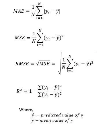
MSE #

measures the average of squared residuals in the dataset

MAE #

measures the average absolute error in the dataset

RMSE #

measures the standard deviation of residuals

Loss Function vs Cost Function #

Loss function:

defined on a single training example
measures how well the model performs on one example

Cost function:

aggregates loss over the whole training set
measures how well the model performs across the dataset

Role of Gradient Descent in Updating the Weights #

Gradient Descent is an optimisation algorithm used to minimise the cost function and find the best-fit line for the model.

Iteratively adjust the weights of the model to reduce the error.
each iteration updates the weights in the direction that minimises the cost function leading to the optimal set of parameters.

References #

Cost Function
/docs/ai/machine-learning/03-gradient-descent-linear-regression/
/docs/ai/machine-learning/03-linear-models-regression/

Home | Machine Learning