Cost Function #

Revision:
A cost function converts model error into a single number. Training means changing the model parameters until this number becomes as small as possible.

Why Cost Function Matters in ML ☆ #

A machine learning model needs a way to decide whether one set of parameters is better than another.

For linear regression, every possible value of the parameters gives a different line. The cost function tells us which line is better by measuring how far the predictions are from the true values.

In simple words:

prediction close to actual value → small error
prediction far from actual value → large error
lower cost → better fit on training data
training objective → minimise the cost

flowchart LR
    A["Training Data"] --> B["Model<br/>with parameters"]
    B --> C["Predictions"]
    C --> D["Compare with<br/>Actual values"]
    D --> E["Cost Function"]
    E --> F["Update Parameters"]
    F --> B

    style A fill:#E1F5FE,stroke:#5b7db1,color:#000
    style B fill:#C8E6C9,stroke:#5f8f6a,color:#000
    style C fill:#FFF9C4,stroke:#b59b3b,color:#000
    style D fill:#EDE7F6,stroke:#8a6fb3,color:#000
    style E fill:#FFF9C4,stroke:#b59b3b,color:#000
    style F fill:#C8E6C9,stroke:#5f8f6a,color:#000

Loss Function, Cost Function and Objective Function ☆ #

These terms are closely related, but they are not exactly the same.

Term	Meaning	Scope
Loss function	Error for one training example	Single data point
Cost function	Average or total loss across the dataset	Whole training set
Objective function	Function we want to minimise or maximise	General optimisation goal

For linear regression, the objective is normally to minimise the cost function.

\[ \text{Training objective} = \min_{w,b} J(w,b) \]

Why Squared Error is Common ☆ #

Squared error is commonly used because:

negative and positive errors do not cancel out
large mistakes are penalised more strongly
the resulting cost surface is smooth
for linear regression, the cost is convex, so there is one global minimum

A low training cost does not always mean the model will generalise well.
If the model is too complex, it may overfit the training data.

also known as an objective function
how far the predicted values are from the actual ones
measure of the difference between predicted values and actual values
quantifies the error between a model’s predicted values and actual values
measures the model’s error on a group of datapoints
method used to predict values by drawing the best-fit line through the data
used to evaluate the accuracy of a model’s predictions
guides the process of adjusting the model’s parameters in order to minimise the difference between predicted and actual values

flowchart TD
CF["Cost<br/>function"] -->|measures| ERR["Prediction<br/>error"]
CF -->|guides| OPT["Optimisation<br/>(training)"]

CF -->|includes| DATA["Data<br/>fit"]
CF -->|may include| PEN["Penalty<br/>(regularisation)"]

style CF fill:#90CAF9,stroke:#1E88E5,color:#000

style ERR fill:#CE93D8,stroke:#8E24AA,color:#000
style OPT fill:#CE93D8,stroke:#8E24AA,color:#000

style DATA fill:#C8E6C9,stroke:#2E7D32,color:#000
style PEN fill:#C8E6C9,stroke:#2E7D32,color:#000

Key takeaway: In ML, we choose model parameters to minimise a cost $J$. For linear regression, the most common choice is the squared error cost.

Training set and model #

You have a training set with:

input features $x$
output targets $y$

The linear regression model is:

\[ f_{w,b}(x)=wx+b \]

The values $w$ and $b$ are the parameters of the model. You adjust them during training to improve the model.

You may also hear:

$w,b$ called coefficients
$w,b$ called weights

What w and b do #

Different values of $w$ and $b$ give different straight lines.

$b$ is the y-intercept: the value of the prediction when $x=0$
$w$ is the slope: how much the prediction changes when $x$ increases

Examples:

If $w=0$ and $b=1.5$: the model predicts a constant $1.5$ (horizontal line)
If $w=0.5$ and $b=0$: the line passes through the origin and has slope $0.5$
If $w=0.5$ and $b=1$: same slope, shifted up by 1

Predictions on training examples #

A training example is written as: $(x^{(i)},y^{(i)})$

For input $x^{(i)}$, the model predicts:

\[ \hat{y}^{(i)} = f_{w,b}\!\left(x^{(i)}\right)=wx^{(i)}+b \] $f_{w,b}\!\left(x^{(i)}\right)$ : our prediction for example $i$ using parameters $w,b$

Goal: choose $w$ and $b$ so that $\hat{y}^{(i)}$ is close to $y^{(i)}$ for many (ideally all) training examples.

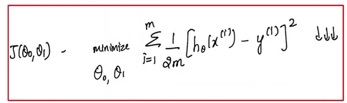
Computing Cost #

Equation for cost with one variable is:

\[ J(w,b)=\frac{1}{2m}\sum_{i=0}^{m-1}\left(f_{w,b}\!\left(x^{(i)}\right)-y^{(i)}\right)^2 \] $\left(f_{w,b}\!\left(x^{(i)}\right)-y^{(i)}\right)^2$ : the squared difference between the target value and the prediction

The squared differences are summed over all the $m$ examples and divided by $2m$ to produce the cost $J(w,b)$

Cost Fn

Intuition: error and squared error #

For one example $i$, the error is:

\[ \hat{y}^{(i)}-y^{(i)} \]

Squared error for example $i$:

\[ \left(\hat{y}^{(i)}-y^{(i)}\right)^2 \]

The cost function sums squared errors over the dataset and averages them (via $2m$).

Squared Error & Mean Squared Error (MSE) #

Feature	Squared Error	Mean Squared Error (MSE)
Scope	Individual data point (residual)	Entire dataset
Formula	$ (y_i - \hat{y}_i)^2 $	$ \frac{1}{n}\sum_{i=1}^{n}(y_i - \hat{y}_i)^2 $
Output	One value per observation	One single value for the model
Purpose	Measures individual error	Measures overall model performance

Cost surface visualisation #

Simplified visualisation: set b=0 #

To build intuition, sometimes we simplify the model by setting $b=0$:

\[ f_w(x)=wx \]

Now the cost depends on one parameter:

\[ J(w)=\frac{1}{2m}\sum_{i=0}^{m-1}\left(wx^{(i)}-y^{(i)}\right)^2 \]

Plotting $J(w)$ versus $w$ gives a U-shaped curve (“bowl”).

Full visualisation: $J(w,b)$ as a surface #

With both parameters $w$ and $b$:

$J(w,b)$ becomes a 3D surface (bowl / hammock shape)
each point $(w,b)$ corresponds to a single value of $J$

Contour plot view #

A contour plot is a 2D way to visualise the same 3D surface:

x-axis: $w$
y-axis: $b$
each contour (oval) shows points with the same cost $J$

The centre of the smallest oval: is the minimum cost point.

Types #

flowchart TD
T["Cost function<br/>types"] --> REG["Regression"]
T --> CLS["Classification"]
T --> PROB["Probabilistic<br/>models"]
T --> REGZ["Regularisation"]

REG --> MSE["MSE"]
REG --> MAE["MAE"]
REG --> HUB["Huber"]

CLS --> CE["Cross-entropy<br/>(log loss)"]
CLS --> HNG["Hinge"]

PROB --> NLL["Negative<br/>log-likelihood"]

REGZ --> L2["L2 (Ridge)"]
REGZ --> L1["L1 (Lasso)"]
REGZ --> EN["Elastic<br/>Net"]

style T fill:#90CAF9,stroke:#1E88E5,color:#000

style REG fill:#C8E6C9,stroke:#2E7D32,color:#000
style CLS fill:#C8E6C9,stroke:#2E7D32,color:#000
style PROB fill:#C8E6C9,stroke:#2E7D32,color:#000
style REGZ fill:#C8E6C9,stroke:#2E7D32,color:#000

style MSE fill:#CE93D8,stroke:#8E24AA,color:#000
style MAE fill:#CE93D8,stroke:#8E24AA,color:#000
style HUB fill:#CE93D8,stroke:#8E24AA,color:#000
style CE fill:#CE93D8,stroke:#8E24AA,color:#000
style HNG fill:#CE93D8,stroke:#8E24AA,color:#000
style NLL fill:#CE93D8,stroke:#8E24AA,color:#000
style L2 fill:#CE93D8,stroke:#8E24AA,color:#000
style L1 fill:#CE93D8,stroke:#8E24AA,color:#000
style EN fill:#CE93D8,stroke:#8E24AA,color:#000

Cost Fn

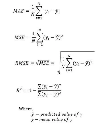
MSE #

measures the average of squared residuals in the dataset

MAE #

measures the average absolute error in the dataset

RMSE #

measures the standard deviation of residuals

Cross-Entropy (Log Loss) #

Used mainly in classification, especially Logistic Regression.

It measures the difference between the predicted probability and the true class label.

Per-example cost:

\[ \mathrm{Cost}\!\left(h_\theta(x),y\right) = -y\log\!\left(h_\theta(x)\right) -(1-y)\log\!\left(1-h_\theta(x)\right) \]

Cost over the full training set:

\[ J(\theta) = -\frac{1}{m}\sum_{i=1}^{m} \left[ y^{(i)}\log\!\left(h_\theta\!\left(x^{(i)}\right)\right) + \left(1-y^{(i)}\right)\log\!\left(1-h_\theta\!\left(x^{(i)}\right)\right) \right] \]

Why it is used:

works well for probabilistic classification
penalises confident wrong predictions heavily
gives a convex optimisation objective for Logistic Regression

Linear vs Logistic (5-Step Comparison) #

Model → Predict → Cost → Gradient → Update

Step	Linear Regression (MSE / Squared Error)	Logistic Regression (Log Loss / Cross-Entropy)
1) Model	$ \hat{y}=wx+b $	$ z=w\cdot x+b,\quad p=\sigma(z)=\frac{1}{1+e^{-z}} $
2) Predict	$ \hat{y}^{(i)}=wx^{(i)}+b $	$ z^{(i)}=w\cdot x^{(i)}+b,\quad p^{(i)}=\sigma(z^{(i)}) $
3) Cost	$ J(w,b)=\frac{1}{2m}\sum_{i=1}^{m}\left(\hat{y}^{(i)}-y^{(i)}\right)^2 $	$ J(w,b)=\frac{1}{m}\sum_{i=1}^{m}\left[-y^{(i)}\log p^{(i)}-(1-y^{(i)})\log(1-p^{(i)})\right] $
4) Gradients	$ \frac{\partial J}{\partial w}=\frac{1}{m}\sum_{i=1}^{m}\left(\hat{y}^{(i)}-y^{(i)}\right)x^{(i)},\quad \frac{\partial J}{\partial b}=\frac{1}{m}\sum_{i=1}^{m}\left(\hat{y}^{(i)}-y^{(i)}\right) $	$ \frac{\partial J}{\partial w}=\frac{1}{m}\sum_{i=1}^{m}\left(p^{(i)}-y^{(i)}\right)x^{(i)},\quad \frac{\partial J}{\partial b}=\frac{1}{m}\sum_{i=1}^{m}\left(p^{(i)}-y^{(i)}\right) $
5) Update	$ w:=w-\alpha\frac{\partial J}{\partial w},\quad b:=b-\alpha\frac{\partial J}{\partial b} $	$ w:=w-\alpha\frac{\partial J}{\partial w},\quad b:=b-\alpha\frac{\partial J}{\partial b} $

Loss Function vs Cost Function #

Loss function:

defined on a single training example
measures how well the model performs on one example

Cost function:

aggregates loss over the whole training set
measures how well the model performs across the dataset

Training objective #

Training means: choose parameters that minimise the cost on the training data.

For regression → cost is often squared error. For classification → a common cost is cross-entropy (log loss).

Role of Gradient Descent in Updating the Weights #

Gradient Descent is an optimisation algorithm used to minimise the cost function and find the best-fit line for the model.

Iteratively adjust the weights of the model to reduce the error.
each iteration updates the weights in the direction that minimises the cost function leading to the optimal set of parameters.

Notes #

Cost function measures model error over the training set.
Linear regression commonly uses squared error.
Logistic regression commonly uses cross-entropy / log loss.
Lower cost usually means better fit on the training data.
Optimisation algorithms such as gradient descent use the cost function to update parameters.

Revision #

Remember this sequence:

\[ \text{Model} \rightarrow \text{Prediction} \rightarrow \text{Error} \rightarrow \text{Cost} \rightarrow \text{Parameter Update} \]

Summary #

A cost function is central to machine learning training. It gives the model a measurable objective. For linear regression, the squared error cost helps us find the best-fit line by minimising prediction errors across the dataset.

References #

Home | Machine Learning

Step	Linear Regression (MSE / Squared Error)	Logistic Regression (Log Loss / Cross-Entropy)
1) Model	\( \hat{y}=wx+b \)	\( z=w\cdot x+b,\quad p=\sigma(z)=\frac{1}{1+e^{-z}} \)
2) Predict	\( \hat{y}^{(i)}=wx^{(i)}+b \)	\( z^{(i)}=w\cdot x^{(i)}+b,\quad p^{(i)}=\sigma(z^{(i)}) \)
3) Cost	\( J(w,b)=\frac{1}{2m}\sum_{i=1}^{m}\left(\hat{y}^{(i)}-y^{(i)}\right)^2 \)	\( J(w,b)=\frac{1}{m}\sum_{i=1}^{m}\left[-y^{(i)}\log p^{(i)}-(1-y^{(i)})\log(1-p^{(i)})\right] \)
4) Gradients	\( \frac{\partial J}{\partial w}=\frac{1}{m}\sum_{i=1}^{m}\left(\hat{y}^{(i)}-y^{(i)}\right)x^{(i)},\quad \frac{\partial J}{\partial b}=\frac{1}{m}\sum_{i=1}^{m}\left(\hat{y}^{(i)}-y^{(i)}\right) \)	\( \frac{\partial J}{\partial w}=\frac{1}{m}\sum_{i=1}^{m}\left(p^{(i)}-y^{(i)}\right)x^{(i)},\quad \frac{\partial J}{\partial b}=\frac{1}{m}\sum_{i=1}^{m}\left(p^{(i)}-y^{(i)}\right) \)
5) Update	\( w:=w-\alpha\frac{\partial J}{\partial w},\quad b:=b-\alpha\frac{\partial J}{\partial b} \)	\( w:=w-\alpha\frac{\partial J}{\partial w},\quad b:=b-\alpha\frac{\partial J}{\partial b} \)