Basic Statistics #
Statistics: describes data (what you see).
Probability: models uncertainty (what you don’t know yet).
- Summarise a dataset using central tendency and variability
- Explain core probability ideas using simple examples
- Apply the axioms of probability
- Distinguish mutually exclusive vs independent events
flowchart TD
    A[Dataset] --> B[Central Tendency]
    A --> C[Variability]
    B --> B1[Mean]
    B --> B2[Median]
    B --> B3[Mode]
    C --> C1[Range]
    C --> C2[Variance]
    C --> C3[Standard Deviation]
    C --> C4[IQR]
Measures of Central Tendency #
Central tendency tells you where the “middle” of the data is. Describes a set of scores with a single number that describes the PERFORMANCE of the group.
Mean (average) #
\[ \bar{x}=\frac{x_1+x_2+\dots+x_n}{n} \]
- Good for: symmetric data without extreme outliers
- Sensitive to: outliers
Median #
The middle value when sorted (or the average of the two middle values).
- Good for: skewed data and outliers
- Often preferred for: income, house prices, anything with long tails
Mode #
The most frequent value.
- Useful for: categorical data (e.g., favourite colour) or repeated discrete values
Rule of thumb:
If your data is skewed, the median usually represents “typical” better than the mean.
Measures of Variability #
Variability tells you: How spread out is the data?
Two datasets can have the same mean, but look completely different if one is tightly packed and the other is widely spread.
That’s why averages alone are never enough.
- Range: “How wide is the data, end to end?”
- Variance: “How much does data vary around the mean?”
- Standard deviation: “Typical distance from the mean?”
- Quartile deviation: “How spread out is the middle 50%?”
Range #
Difference between the largest and smallest value.
\[ \text{Range}=\max(x)-\min(x) \]
Simple but fragile (a single outlier can dominate):
- It only uses two values
- One extreme outlier can distort it
Variance #
Variance measures how far values are from the mean, on average (squared).
\[ s^2=\frac{\sum_{i=1}^{n}(x_i-\bar{x})^2}{n-1} \]
Take each value and subtract the mean
Square the distance (removes negatives and penalises big deviations)
Average the squared distances
High variance → data points are spread far apart.
Low variance → data points are tightly clustered near the mean.
Variance is in squared units, so it can be harder to interpret directly.
Population Variance #
Population variance equals mean (average) squared deviation (distance) of the scores from the population mean
Variance is the average of squared deviations, so we identify population variance with a lowercase Greek letter sigma squared: σ^2
Standard deviation is the square root of the variance, so we identify it with a lowercase Greek letter sigma: σ
Standard Deviation #
Standard deviation is the square root of variance.
\[ s=\sqrt{s^2} \]
- Same units as the data
- Small SD → data is consistent
- Large SD → data is spread out
Quartiles, IQR, and Quartile Deviation #
Quartiles split sorted data into four equal parts:
- Q1: 25% of data lies below it
- Q3: 75% of data lies below it
Interquartile Range (IQR):
- It is measure of Variation
- Also Known as Mid-spread : Spread in the Middle 50%
- Difference Between Third & First Quartiles:
- Not Affected by Extreme Values
\[ \text{IQR}=Q_3-Q_1 \]
Quartile Deviation (QD) is half the IQR:
\[ \text{QD}=\frac{\text{IQR}}{2} \]
- Robust to (not affected by) outliers
- Great for skewed distributions (e.g., income, house prices)
Five-number summary #
A compact description of a dataset using five values:
- Minimum → where the data begins.
- Q1 → the middle of the lower half of the data.
- Median → splits the data into two equal halves.
- Q3 → middle of the upper half of the data.
- Maximum → where the data ends.
With one simple visual, you can immediately see:
- Spread
- Skewness
- Outliers (potentially)
- How datasets compare
This is the backbone of the box-and-whisker plot.
Box-and-Whisker Plot #
Structure of a box plot using the five-number summary.
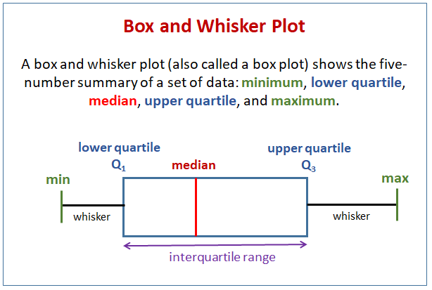
In a real box plot:
- The box spans from Q1 to Q3
- The line inside the box is the median
- The whiskers extend towards the minimum and maximum (or to non-outlier limits)