Formula Sheet

March 12, 2026

Formula Sheet #

This page is a quick reference of definitions + formulas, grouped by the modules.

Notation #

• Sample size: \( n \) (sample), \( N \) (population)
• Sample mean: \( \bar{x} \) , population mean: \( \mu \)
• Sample variance: \( s^2 \) , population variance: \( \sigma^2 \)
• Sample SD: \( s \) , population SD: \( \sigma \)
• Complement: \( A^c \)
• Intersection (“and”): \( A\cap B \) , union (“or”): \( A\cup B \)
• Conditional probability: \( P(A\mid B) \)

1. Basic Probability & Statistics #

1.1 Measures of Central Tendency #

Arithmetic mean #

Sample mean (ungrouped):

Supervised Learning

January 3, 2026

Supervised Learning #

Trained using labelled data.
Each example in the training set includes the correct output.
The algorithm learns to generalise and make predictions on unseen data.
Generally more accurate than unsupervised methods.
Requires human intervention for labelling and setup.
Widely used due to its accuracy and efficiency.
Produces highly accurate results when trained on good-quality labelled data.

Classification #

Output is discrete (e.g. Yes/No, Spam/Not Spam).
Used for categorising data into predefined classes.
Support Vector Machine (SVM) is a common classifier (a linear classifier with margin-based separation).

Artificial Intelligence

July 4, 2024

My AI Notes #

Learning how machines learn! My working notes as I learn AI.

flowchart LR
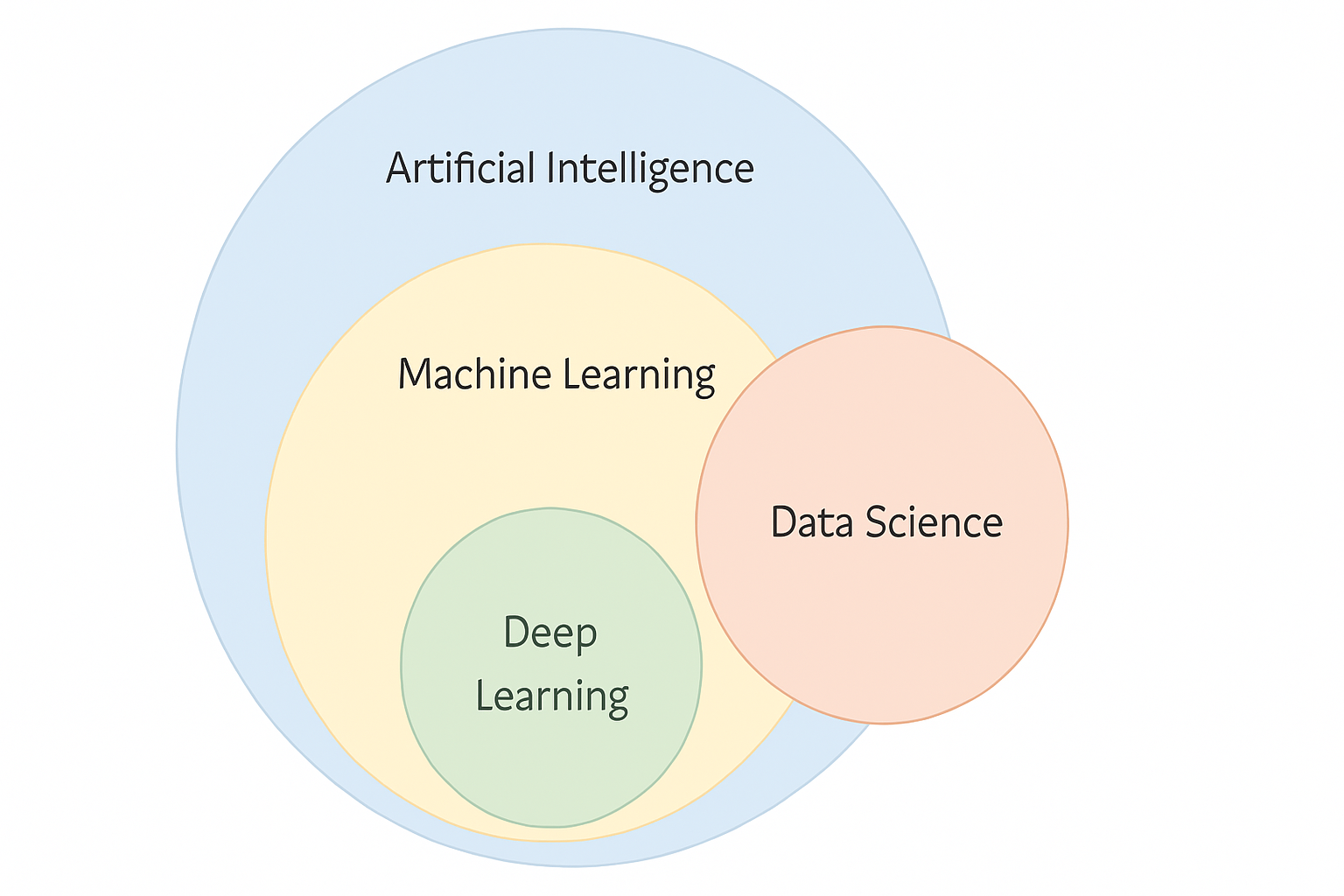
    AI[Artificial Intelligence]
    ML[Machine Learning]
    DL[Deep Learning]
    FM[Foundation Models]
    LLM[LLM Models]

    AI --> ML
    ML --> DL
    DL --> FM
    FM --> LLM

    style AI fill:#E1F5FE
    style ML fill:#C8E6C9
    style DL fill:#90CAF9
    style FM fill:#64B5F6
    style LLM fill:#FFCCBC

• Mathematical Foundations for Machine Learning
• Statistical Methods
• Machine Learning
• Deep Neural Networks

• AI Foundation
  • AI Stages: ANI, AGI, ASI
  • AI Stack
  • AI Pipeline
  • AI Learning Resources
• Machine Learning
  • Supervised Learning
  • Unsupervised Learning
  • Semi-Supervised Learning
  • Reinforcement Learning
  • ML Workflow
  • Regression(Linear Models)
  • Ordinary Least Squares
  • Cost Function
  • Gradient Descent
  • Classification(Linear Models)
  • Decision Tree
  • Instance-based Learning
  • Instance-based Learning
  • Support Vector Machine
  • Bayesian Learning
  • Ensemble Learning
  • Evaluation/Comparison
  • ML Pipeline
• Generative AI
  • Foundation Models
  • LLM - Model
  • AI Agents
  • Retrieval-Augmented Generation (RAG)
• Deep Learning
  • Neural Networks
  • Artificial Neuron and Perceptron
  • LNN for Regression
  • Gradient Descent Algorithm
  • LNN for Classification
  • Deep Feedforward Neural Networks (DFNN) for Classification
  • Convolutional Neural Networks
  • Deep CNN Architectures
  • CNN Pipeline
  • Recurrent Neural Networks
  • Deep Recurrent Neural Networks
  • Attention Mechanism
  • Transformer
  • Optimisation of Deep models
  • Regularisation for Deep models
• Mathematical Foundation
  • Linear Algebra
    • Linear Systems
      • Systems of Linear Equations
      • Matrices
      • Matrix Transposition
      • Solving Linear Systems
      • Forward and Backward Substitution
      • Inverse Matrix
      • Convex Combination
    • Vector Spaces
      • Basis and Rank
      • Linear Independence
      • Norm
      • Inner Products and Dot Product
      • Lengths and Distances
      • Angles and Orthogonality
      • Orthonormal Basis
      • Feature Space
      • Cauchy–Schwarz
    • Matrix Decompositions
      • Special Matrices
      • Characteristic Polynomial
      • Determinant and Trace
      • Eigenvalues and Eigenvectors
      • Cholesky Decomposition
      • Eigen Decomposition
      • Diagonalization
      • Singular Value Decomposition (SVD)
      • Matrix Approximation
    • Dimensionality reduction and PCA
      • Principal Component Analysis (PCA)
      • PCA Theory
      • PCA in Practice
      • Latent Variable Perspective
      • Mathematical Preliminaries of SVM
      • Nonlinear SVM and Kernels
  • Calculus
    • Vector Calculus
      • Differentiation of Univariate Functions
      • Partial Differentiation and Gradients
      • Gradients of Vector-Valued and Matrix Functions
      • Useful Gradient Identities
      • Backpropagation and Automatic Differentiation
      • Higher-order derivatives
      • Taylor’s series
      • Maxima and Minima
    • Continuous Optimisation
      • Optimisation using Gradient Descent
      • Constrained Optimisation
      • Lagrange Multipliers
      • Convex Optimisation
    • Nonlinear Optimisation
      • Challenges in Gradient-Based Optimisation
      • Stochastic Gradient Descent (SGD)
      • Momentum-Based Learning
      • Adaptive Methods: AdaGrad, RMSProp, Adam
      • Tuning Hyperparameters and Preprocessing
• Statistics
  • Formula Sheet
  • Stats Formula Sheet
  • Basic Statistics
  • Basic Probability
  • Hypothesis Testing
  • Prediction & Forecasting
  • Gaussian Mixture model & Expectation Maximization
  • Conditional Probability & Bayes’ Theorem
    • Conditional Probability
    • Bayes’ Theorem
    • Naïve Bayes
  • Probability Distributions
    • Random Variables
    • Common Probability Distributions

• Machine Learning → The broad field where systems learn patterns from data to make predictions or decisions.
• Neural Networks → A subset of machine learning that uses interconnected artificial neurons to model complex relationships.
• Deep Learning → A subset of neural networks that uses many hidden layers to learn high-level features from large datasets.
• Foundation Models → Large deep learning models trained on massive datasets and reused across many tasks using transfer learning.
• LLMs (Large Language Models) → A specialised type of foundation model focused on understanding and generating human language.

flowchart TD
AI["Artificial<br/>Intelligence"]
ML["Machine<br/>Learning"]
NN["Neural<br/>Networks"]
DL["Deep<br/>Learning"]
FM["Foundation<br/>Models"]
LLM["LLM<br/>Models"]

AI --> ML
ML --> NN
NN --> DL
DL --> FM
FM --> LLM

LR["Linear<br/>Regression"]
DT["Decision<br/>Trees"]
ML --> LR
ML --> DT

MLP["MLP"]
CNN["CNN"]
NN --> MLP
NN --> CNN

CNNDL["CNN<br/>(deep)"]
RNN["RNN"]
DL --> CNNDL
DL --> RNN

BERT["BERT"]
CLIP["CLIP"]
FM --> BERT
FM --> CLIP

GPT["GPT"]
LLAMA["LLaMA"]
LLM --> GPT
LLM --> LLAMA

TEXT["Text"]
IMAGE["Images"]
AUDIO["Audio"]
VIDEO["Video"]
LLM --> TEXT
LLM --> IMAGE
LLM --> AUDIO
LLM --> VIDEO

style AI fill:#90CAF9,stroke:#1E88E5,color:#000
style ML fill:#90CAF9,stroke:#1E88E5,color:#000
style NN fill:#90CAF9,stroke:#1E88E5,color:#000

style DL fill:#CE93D8,stroke:#8E24AA,color:#000
style FM fill:#CE93D8,stroke:#8E24AA,color:#000

style LLM fill:#C8E6C9,stroke:#2E7D32,color:#000
style LR fill:#C8E6C9,stroke:#2E7D32,color:#000
style DT fill:#C8E6C9,stroke:#2E7D32,color:#000
style MLP fill:#C8E6C9,stroke:#2E7D32,color:#000
style CNN fill:#C8E6C9,stroke:#2E7D32,color:#000
style CNNDL fill:#C8E6C9,stroke:#2E7D32,color:#000
style RNN fill:#C8E6C9,stroke:#2E7D32,color:#000
style BERT fill:#C8E6C9,stroke:#2E7D32,color:#000
style CLIP fill:#C8E6C9,stroke:#2E7D32,color:#000
style GPT fill:#C8E6C9,stroke:#2E7D32,color:#000
style LLAMA fill:#C8E6C9,stroke:#2E7D32,color:#000
style TEXT fill:#C8E6C9,stroke:#2E7D32,color:#000
style IMAGE fill:#C8E6C9,stroke:#2E7D32,color:#000
style AUDIO fill:#C8E6C9,stroke:#2E7D32,color:#000
style VIDEO fill:#C8E6C9,stroke:#2E7D32,color:#000

Stats Formula Sheet

February 25, 2026

Stats Formula Sheet #

Keep this page as a quick reference of definitions + formulas.

Notation #

• Sample size: \( n \) (sample), \( N \) (population)
• Mean: \( \bar{x} \) (sample), \( \mu \) (population)
• Variance: \( s^2 \) (sample), \( \sigma^2 \) (population)
• Standard deviation: \( s \) (sample), \( \sigma \) (population)

Module 1: Basic Statistics #

Measures of Central Tendency #

Sample mean (ungrouped):

Unsupervised Learning

January 3, 2026

Unsupervised Learning #

• Works on unlabelled raw data.
• The algorithm discovers hidden patterns without prior knowledge of outcomes.
• Requires no human intervention during training.
• Does not make direct predictions — it groups or organises data instead.
• Carries a higher risk because there’s no ground truth to verify results.
• Common techniques include Clustering, Association, and Dimensionality Reduction.

stateDiagram-v2

  %% ML maths-based colours (same palette as supervised)
  classDef probability fill:#d1fae5,stroke:#065f46,stroke-width:1px
  classDef geometry fill:#ffedd5,stroke:#9a3412,stroke-width:1px
  classDef category font-style:italic,font-weight:bold,fill:#f3f4f6,stroke:#374151

  %% Root
  USL: Unsupervised Learning

  %% Main branches
  USL --> CLU:::category
  CLU: Clustering

  USL --> DR:::category
  DR: Dimensionality Reduction

  %% Clustering algorithms
  CLU --> KM:::geometry
  KM: K-Means

  CLU --> HC:::geometry
  HC: Hierarchical Clustering

  CLU --> DB:::geometry
  DB: DBSCAN

  %% Probabilistic models
  USL --> PM:::category
  PM: Probabilistic Models

  PM --> GMM:::probability
  GMM: Gaussian Mixture Model

  PM --> HMM:::probability
  HMM: Hidden Markov Model

Clustering #

• Groups similar data points together based on shared features.
• Commonly used for market segmentation, image compression, and anomaly detection.

Common Types of Clustering #

• K-Means Clustering – Divides data into K groups based on similarity.
• Hierarchical Clustering – Builds a hierarchy (tree) of clusters.
• DBSCAN (Density-Based Spatial Clustering) – Groups points close in density; identifies noise/outliers.

Association #

• Identifies relationships or correlations between variables in a dataset.
• Commonly used in market basket analysis (e.g. “Customers who bought X also bought Y”).

Common Techniques #

• Apriori Algorithm – Finds frequent itemsets and generates association rules.
• Eclat Algorithm – Similar to Apriori but uses set intersections for faster computation.

Dimensionality Reduction #

• Reduces the number of input variables to simplify data.
• Helps remove noise and redundancy.
• Commonly used in data pre-processing and visualisation.

Common Techniques #

• Principal Component Analysis (PCA) – Projects data onto fewer dimensions while keeping most variance.
• Linear Discriminant Analysis (LDA) – Focuses on class separation.
• t-SNE (t-Distributed Stochastic Neighbour Embedding) – Used for visualising high-dimensional data.
• Autoencoders – Neural networks that compress and reconstruct data.

mindmap
  root(Unsupervised Learning)
    Clustering
      K Means
      Hierarchical Clustering
      DBSCAN
    Dimensionality Reduction
      PCA
      t SNE
      Autoencoders
    Probabilistic Models
      Gaussian Mixture Model
      Hidden Markov Model

Home | Machine Learning

Semi-Supervised Learning

January 3, 2026

Semi-Supervised Learning #

• A combination of labelled and unlabelled data.
• Useful when labelling large datasets is expensive or time-consuming.
• Works well with high-volume datasets (e.g. millions of images).
• Only a small fraction of data is labelled (e.g. a few thousand).
• The algorithm learns from both labelled examples and structure in unlabelled data.
• Ideal for medical imaging where labelled data is limited.
• For example, a radiologist can label a small set of medical scans,
  and the model uses that to learn from thousands of unlabelled scans.
• Helps improve accuracy and generalisation with minimal manual effort.

Home | Machine Learning

Reinforcement Learning

Reinforcement Learning (RL) #

RL is learning by trial and error.

Reinforcement Learning (RL) is a type of machine learning where an autonomous agent learns to make decisions by interacting with an environment.

Instead of being told the correct answer, the agent:

• takes actions
• observes outcomes
• receives rewards or penalties
• gradually learns a strategy that maximises long-term reward

Reinforcement Learning teaches an agent how to act, not what to predict.

AI Foundation

January 26, 2026

AI #

A selection of notes that didn’t fit elsewhere or are being worked on!.

• AI Stages: ANI, AGI, ASI
• AI Stack
• AI Pipeline
• AI Learning Resources

AI Stages: ANI, AGI, ASI

July 4, 2024

AI Development Stages: ANI → AGI → ASI #

Artificial Intelligence is often described in three stages, based on capability and scope:

• ANI: Task-specific intelligence (today’s AI)
• AGI: Human-level general intelligence (future goal)
• ASI: Beyond human intelligence (theoretical)

ANI — Artificial Narrow Intelligence #

• also called Weak AI
• designed to perform one specific task
• Operates within a predefined environment
• Cannot generalise beyond its training
• Most AI systems today are ANI

examples

Basic Statistics

Basic Statistics #

Statistics: describes data (what you see).
Probability: models uncertainty (what you don’t know yet).

• Summarise a dataset using central tendency and variability
• Explain core probability ideas using simple examples
• Apply the axioms of probability
• Distinguish mutually exclusive vs independent events

flowchart TD
    A[Dataset] --> B[Central Tendency]
    A --> C[Variability]
    B --> B1[Mean]
    B --> B2[Median]
    B --> B3[Mode]
    C --> C1[Range]
    C --> C2[Variance]
    C --> C3[Standard Deviation]
    C --> C4[IQR]

Measures of Central Tendency #

Central tendency tells you where the “middle” of the data is. Describes a set of scores with a single number that describes the PERFORMANCE of the group.